Observable to standalone
The map below was initially developed as a standard Observable notebook. It was then transformed into a standalone application using the observable-to-standalone bundle methodology that we describe in this post. The code is available at https://github.com/Fil/SphericalContoursStandalone.

The methodology uses yarn (or npm), and follows four steps:
- Step 1. Retrieve a local copy of the notebook
- Step 2. Play the selected cell(s) in the HTML document
- Step 3. Route require(module) to
node_modules/. - Step 4. Route data URLs to locally hosted versions
At the end of the procedure, you will have a copy of the notebook and a
copy of its dependencies in node_modules/. The JavaScript code will be
bundled and compressed, with a source-map, in the public/ directory,
together with any other assets you have in src/ and a downloaded copy of
your data files. All ready to be served with a local web server, or
deployed to a static host.
public
├── data
│   ├── 110m_land.geojson
│   └── points.json
├── favicon.ico
├── index.html
├── main.js
├── main.min.js
└── main.min.js.map
Step 1. Retrieve a local copy of the notebook
To do so, the notebook must be shared. Its “tarball” address (given in the
“Download code” option of the `…` menu) will be written in the package.json
file that describes the node project, in the notebook field:
"notebook": "https://api.observablehq.com/@fil/spherical-contours.tgz?v=3",
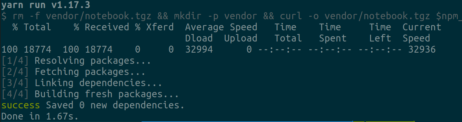
Once this is ready, each call to yarn notebook will download the latest shared
(or in this case, published) version of the notebook:
Step 2. Play the selected cell(s) in the HTML document
Edit src/render.js to map named cells to HTML elements; for example:
case 'chart':
  return new Inspector(document.querySelector('#chart'))
will render the notebook cell named “chart” into index.html’s
<div id="chart"></div>.
Step 3. Route require(module) to node_modules.
To do so, you need to check the exact way the modules are required in
your notebook (and its imports). Then adapt the contents of
src/customResolve.js so that these modules are loaded from their local
versions.
import { require } from 'd3-require'
import * as d3 from 'd3'
import * as d3GeoVoronoi from 'd3-geo-voronoi'
import * as d3GeoProjection from 'd3-geo-projection'

// Resolve "d3@5" module to current object `d3`
export const customResolve = require.alias({
  'd3@5': d3,
  'd3-geo-voronoi@1.5': d3GeoVoronoi,
  'd3-geo-projection@2': d3GeoProjection,
}).resolve
The modules must also be added to the project under the same version
with yarn add --dev ….
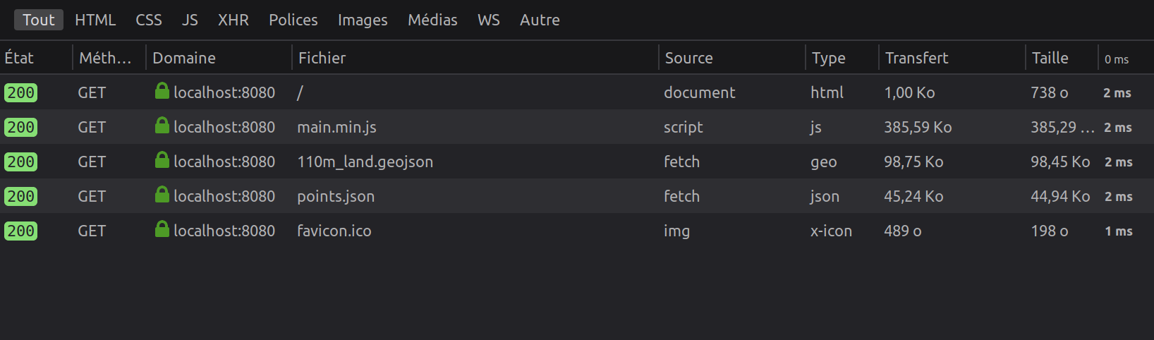
If you forget to specify a module, or if its name is spelled differently in the require() cells of your notebook, your project will load it from the Internet. So double check in your browser’s Network inspector tab to make sure everything is loaded locally.
Step 4. Route data URLs to locally hosted versions
If you want the cells containing d3.json("https://…") or d3.csv("https://…") to use a local copy of those resources, you can specify the files URLs and local names in the fetchAlias.json map:
{
  "https://gist.githubusercontent.com/Fil/6bc…/points.json": "data/points.json",
  "https://unpkg.com/vis…/110m_land.geojson": "data/110m_land.geojson"
}
Again, if you forget to specify a resource’s URL, for example after changing it in your source notebook, the data will be loaded from the Internet.
Congratulations!
If you did all these steps for all the “remote” files, your project is now fully standalone, and can be served with a local webserver with no Internet connection.