The performance metric

You need to cite the following journal paper in all publications including results for which you used the LIRIS dataset:.

C Wolf, J. Mille, E. Lombardi, O. Celiktutan, M. Jiu, E. Dogan, G. Eren, M. Baccouche, E. Dellandrea, C.-E. Bichot, C. Garcia, B. Sankur, Evaluation of video activity localizations integrating quality and quantity measurements, In Computer Vision and Image Understanding (127):14-30, 2014.

The metric

The goal of the evaluation scheme is to measure a match between the annotated ground-truth and a result, i.e. between:

a list of ground truth actions $G^{v,a}$ , where $G^{v,a}$ corresponds to the $a^{th}$ action in the $v^{th}$ video and where each action consists of a set of bounding boxes $G^{v,a}_b$ marked with the same class.
a list of detected actions $D^{v,a}$ , where $D^{v,a}$ corresponds to the $a^{th}$ action in the $v^{th}$ video and where each action consists of a set of bounding boxes $D^{v,a}_b$ marked with the same class.

The objective is to measure the degree of similarity between the two lists. The measure should penalize information loss, which occurs if actions or (spatial or temporal) parts of actions have not been detected, and it should penalize information clutter, i.e. false alarms or detections which are (spatially or temporally) larger than necessary. As in our object recognition measure [1], we designed the metric to fulfill the following goals:

The metric should provide a quantitative evaluation: the evaluation measure should intuitively tell how many actions have been detected correctly, and how many false alarms have been created.
The metric should provide a qualitative evaluation: it should give an easy interpretation of the detection quality.

There is a contradiction between goal (1), to be able to count the number of detected actions, and goal (2), to be able to measure detection quality. Indeed, the two goals are related: the number of actions we consider as detected depends on the quality requirements which we impose for a single action in order to be considered as detected. For this reason we propose a natural way to combine these two goals:

We provide traditional precision and recall values measuring detection quantity. An action is considered to be correctly detected or not with two fixed thresholds on the amount of overlap between a ground truth action and a detected action.
We complete the metric with plots which illustrate the dependence of quantity on quality. These performance graphs, similar to the graphs proposed in [1], visually describe the behavior of a detection algorithm.

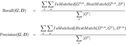
The first measure, Recall, describes how many action occurrences have been correctly detected, with respect to the total number of action occurrences in the dataset, whereas the second measure, Precision, describes how much unnecessary false alarms the system produces, i.e. how many detected actions are matched with respect to the total number of detected actions:

$\begin{displaymath} \begin{array}{ccc} \textrm{Recall} (\mbox{\boldmath$G$},\mbo... ...nd actions}} {\textrm{Number of found actions}} \\ \end{array}\end{displaymath}$

(1)

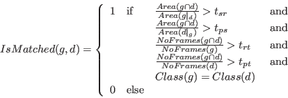
Of course this definition depends on the criteria we impose on action to be considered as correctly found. How close do the detected bounding boxes need to be to the ground truth bounding boxes, how close does the found temporal duration of the action need to be to the duration in the ground truth? How about multiple detections for a single ground truth action and vice versa? An intuitive way to decide this is the following definition:

$\begin{displaymath} \begin{array}{ccc} \textrm{Recall} (\mbox{\boldmath$G$},\mbo... ...{v,a})}} {\displaystyle{\sum_v \vert D^v\vert}} \\ \end{array}\end{displaymath}$

(2)

Both measures rely on finding a best matching action in a list for a given action; Recall matches each action of the ground truth to one of the actions in the detection list, whereas Precision matches each action of the detected list to one of the actions in the ground truth list. This is done in two steps:

For a single action, the functions finds the best match in the respective other list (detections or ground truth).
For a pair of actions (detection and ground gruth), decides whether this correspondence satisfies our criteria on geometric and temporal overlap.

The

function finds the best match for an action in a list of potential candidate matches. It maximizes the normalized overlap between the two actions over all frames:

$\begin{displaymath} BestMatch (X^{v,a},Y^v) = \displaystyle{\arg \max_{a'=1\ldot... ...ot Area(X^{v,a} \cap Y^{v,a'})}{Area(X^{v,a})+Area(Y^{v,a'})}} \end{displaymath}$

(3)

decides whether a matched action is sufficiently matched based on four criteria, two of which are spatial and two are temporal. We first describe the criteria intuitively and then formalize them in equation (4). A detected action is matched to a ground truth action if all of the following criteria are satisfied :

they have the same action class, and
the size of the overlap of the bounding boxes is sufficiently large with respect to the size of the bounding boxes in the ground truth set, i.e. a sufficiently large portion of the ground truth rectangles is correctly found. In order to ignore temporal differences, this calculation includes only frames which are part of both actions, detected and ground truth.
the size of the overlap of the bounding boxes is sufficiently large with respect to the size of the bounding boxes in the detected set, i.e. the space detected in excess is sufficiently small. In order to ignore temporal differences, this calculation includes only frames which are part of both actions, detected and ground truth.
the number of frames which are part of both actions is sufficiently large with respect to the number frames in the ground truth set, i.e. a sufficiently long duration of the action has been found.
the number of frames which are part of both actions is sufficiently large with respect to the number frames in the detected set, i.e. the detected excess duration is sufficiently small.

To give a formal expression for this criteria we we abbreviate the ground truth action by $g=G^{v,a}$ and the detected action by $d=D^{v,a'}$ . Furthermore, we denote by $g\vert _d$ the set of bounding boxes of the ground truth action

restricted to uniquely the frames which are also part of detected action

. In a similar way, we denote by $d\vert _g$ the set of bounding boxes of the detection action

restricted to uniquely the frames which are also part of ground truth action

. Then, the criteria are given as

$\begin{displaymath} IsMatched(g,d) = \left \{ \begin{array}{llll} 1 & \textrm{i... ...ss(g) = Class(d) \\ 0 & \textrm{else} \\ \end{array}\right . \end{displaymath}$

(4)

where

is the sum of the areas of the bounding boxes of set

and $\cap$ is the intersection operator returning the overlap of two bounding boxes.

is the number of frames in set

Ranking

In order to get a single measure, recall and precision are combined into the traditional F-score (or harmonic mean), introduced by the information retrieval community [2]. Its advantage is that the minimum of the two performance values is emphasized:

$\begin{displaymath} F = \frac{2\cdot Precion \cdot Recall}{Precision+Recall} \end{displaymath}$

(5)

However, this measure still depends on the matching quality criteria we choose, i.e. on the thresholds $t_{sr}, t_{ps}, t_{rt}, t_{pt}$ . The final measure integrates the performance over the whole range of matching criteria, by varying these constraints. Four measures are created, each one measuring the performance while varying one of the thresholds while keeping the other ones fixed at a very low value ( $\epsilon=0.1$ ). Denoting by $F(t_{sr},t_{ps},t_{rt},t_{pt})$ the F-Score of equation (5) depending on the quality constraints, we get:

$\begin{displaymath} \begin{array}{l} I_{sr} = \frac{1}{N} F(t_{rs},\epsilon,\eps... ...frac{1}{N} F(\epsilon,\epsilon,\epsilon,t_{pt}) \\ \end{array}\end{displaymath}$

(6)

where

is value specifying the number of samples for the numerical integration. The value used for ranking is the mean over these four values:

$\begin{displaymath} IntegratedPerformance = \frac{1}{4} (I_{rs} + I_{ps} + I_{rt} + I_{pt}) \end{displaymath}$

(7)

Performance vs. quality curves

As mentioned above, we complete the performance measures by visual graphs which illustrate the dependence of quantity (precision and recall) on detection quality requirements. These performance graphs, similar to the graphs proposed in [1], are related to the integral measures in equation (6) and visually describe the behavior of a detection algorithm. More precisely, the integral measures each correspond to the mean value of one of the proposed performance curves. Figure 1c shows example graphs. The left graph shows Precision, Recall and the harmonic mean with respect to the varying constraint $t_{rs}$ (spatial recall), while the other thresholds are kept constant and fixed to a low value $\epsilon$ . The graph shows that the example method tends to completely localize the actions, since more than 60% of the actions are detected even if a complete coverage of the ground truth action by the detected action is required (). If the requirement is relaxed to 80% () then more than 90% of the actions are recalled.

The right graph shows Precision and Recall with respect to varying constraint $t_{tp}$ (temporal precision) while the other thresholds are kept constant. The graph shows that the example method tends to detect actions longer than necessary, since Recall and Precision drop to zero if $t_{pt}=1$ , which means that no additional detected duration is tolerated. 90% of the actions are detected if 50% of the additional duration area is allowed ( $t_{pt}=0.5$ ).

Confusion matrices

The proposed competition requires the participants to go beyond classification, as the tasks also require detection and localization. However, it might be interesting to complete the traditional precision and recall measures with a confusion matrix which illustrates the pure classification performance of the participants' methods. This can be done easily by associating a detected action to each ground truth rectangle using equations (2) and (3), while removing the class equality constraint from (3). The pairs ground truth -- result actions can be used to calculate a confusion matrix, shown in the following example:

Note that the confusion matrix ignores actions which have not been detected, actions with no result. Therefore, unlike in classification tasks, the recognition rate (accuracy) can not be determined from its diagonal. For this reason the confusion matrix must be accompanied by precision and recall values.

References

[1] C. Wolf and J.-M. Jolion, Object count/Area Graphs for the Evaluation of Object Detection and Segmentation Algorithms, in International Journal on Document Analysis and Recognition , 8(4):280-296, 2006. [PDF]

[2] C.J. van Rijsbergen. Information Retrieval. Butterworths, London, 2nd edition, 1979.

Organization, contact

The dataset was collected and produced by members of the LIRIS Laboratory, CNRS, France
Christian Wolf, Julien Mille, Eric Lombardi, Bülent Sankur (BUSIM, Bogazici University, Turkey), Emmanuel Dellandréa, Christophe Garcia, Charles-Edmond Bichot, Mingyuan Jiu, Oya Celiktutan, Moez Baccouche

Send questions to christian.wolf (at) liris.cnrs.fr